glmmSeq

The aim of this package is to model gene expression with a general linear mixed model (GLMM) as described in the R4RA study [1]. The most widely used mainstream differential gene expression analysis tools (e.g Limma, DESeq2, edgeR) are all unable to fit mixed effects linear models. This package however fits negative binomial mixed effects models at individual gene level using the negative.binomial function from MASS and the glmer function in lme4 which enables random effect, as as well as mixed effects, to be modelled.

Installing from CRAN

install.packages("glmmSeq")

Installing from Github

devtools::install_github("myles-lewis/glmmSeq")

Installing Locally

Or you can source the functions individually:

functions = list.files("./R", full.names = TRUE)
invisible(lapply(functions, source))

But you will need to load in the additional libraries:

# Install CRAN packages
invisible(lapply(c("MASS", "car", "ggplot2", "ggpubr", "lme4","lmerTest",
                   "methods", "parallel", "plotly", "pbapply", "pbmcapply"),
                 function(p){
                   if(! p %in% rownames(installed.packages())) {
                     install.packages(p)
                   }
                   library(p, character.only=TRUE)
                 }))

# Install BioConductor packages
if (!requireNamespace("BiocManager", quietly = TRUE))
  install.packages("BiocManager")
invisible(lapply(c("qvalue"), function(p){
  if(! p %in% rownames(installed.packages())) BiocManager::install(p)
  library(p, character.only=TRUE)
}))

Overview

To get started, first we load in the package:

library(glmmSeq)
set.seed(1234)

This vignette will demonstrate the power of this package using a minimal example from the PEAC data set. Here we focus on the synovial biopsy RNA-Seq data from this cohort of patients with early rheumatoid arthritis.

data(PEAC_minimal_load)

This data contains:

metadata: which describes each sample. Including patient ID, sample time-point, and six-month EULAR response. Where EULAR is a rheumatoid arthritis response metric based on composite DAS28 scores.
tpm: the transcript per million RNA-seq count data

These are outlined in the following subsections.

Metadata

metadata$EULAR_binary  = NA
metadata$EULAR_binary[metadata$EULAR_6m %in%
                        c("Good", "Moderate" )] = "responder"
metadata$EULAR_binary[metadata$EULAR_6m %in% c("Non-response")] = "non_responder"

kable(head(metadata), row.names = F) %>% kable_styling()

PATID	Timepoint	EULAR_6m	EULAR_binary
PAT300	6	Good	responder
PAT209	6	Good	responder
PAT219	6	Moderate	responder
PAT211	6	Good	responder
PAT216	6	Good	responder
PAT212	6	Good	responder

Count data

kable(head(tpm)) %>% kable_styling() %>%
  scroll_box(width = "100%")

	S9001	S9002	S9003	S9004	S9006	S9007	S9008	S9009	S9010	S9011	S9012	S9013	S9014	S9016	S9017	S9018	S9019	S9020	S9021	S9023	S9025	S9029	S9034	S9035	S9036	S9038	S9039	S9040	S9042	S9043	S9044	S9045	S9047	S9048	S9049	S9052	S9053	S9054	S9056	S9059	S9060	S9063	S9065	S9066	S9067	S9068	S9069	S9070	S9072	S9073	S9074	S9075	S9076	S9077	S9078	S9079	S9080	S9081	S9083	S9084	S9085	S9086	S9087	S9088	S9089	S9090	S9091	S9092	S9093	S9094	S9095	S9096	S9097	S9098	S9099	S9100	S9101	S9102	S9103	S9104	S9105	S9106	S9107	S9108	S9109	S9110	S9111	S9112	S9113	S9114	S9115	S9116	S9117	S9119	S9120	S9121	S9122	S9123	S9124	S9125	S9127	S9128	S9129	S9130	S9131	S9132	S9133	S9134	S9135	S9136	S9137	S9138	S9139	S9140	S9141	S9142	S9143	S9144	S9145	S9146	S9147	S9148	S9149
MS4A1	1.622818	2.024451	0.6995153	15.742876	2.123731	57.280078	2.011160	0.580000	1.006783	0.391420	3.886618	2.746742	31.647637	20.16757	0.925393	3.4271907	3.130648	1.422480	63.14643	0.295537	12.7877279	4.817494	15.874491	0.569317	4.429667	1.060991	2.1850700	5.321541	3.542383	1.676829	5.471954	29.942195	4.5519540	7.252108	1.9540320	12.947362	73.430132	2.364819	5.2372870	12.281007	17.637846	72.557856	2.379427	0.444729	89.042394	2.4190970	226.612930	8.01254	5.328680	0.7414830	4.669566	5.218332	0.0676825	26.0579080	77.100135	23.2918620	50.306168	5.24953	1.342645	0.511810	0.2428008	7.756002	1.020052	0.602854	0.2444728	2.047680	2.110914	0.683498	24.664095	1.9789030	0.1702800	3.910493	6.5513870	0.8342158	31.7618280	1.136854	17.98745	3.369558	8.577294	1.453945	41.031738	42.991580	27.58865	14.876902	21.6405734	42.049748	75.6557000	2.501497	3.560322	32.1091249	7.008288	0.746264	10.0969886	92.3355460	0.5157370	0.8011538	5.075003	1.979931	0.2068106	2.717007	0.984857	0.7771422	0.000000	8.2769093	1.261793	2.361150	2.372850	0.6968002	43.9459380	5.0257346	0.281387	0.4190982	1.716238	16.25508	1.9852750	26.591585	27.994183	1.325606	1.323197	12.47092	2.3049434	1.4901770	0.229867
ADAM12	2.581805	1.110548	0.9573992	5.466742	2.645153	0.972897	0.658545	1.159264	0.462860	3.074193	10.947068	9.678026	1.205472	11.63376	1.772810	0.3506414	3.528288	17.416140	6.36844	4.064450	0.2666618	2.113812	0.473972	1.222569	30.012798	0.181003	2.4554526	4.136035	13.961315	4.195791	3.629029	8.362213	0.6999296	7.894137	0.3268513	2.847538	7.015717	0.717947	0.4396555	1.141057	1.069326	1.895644	0.486478	14.504778	1.897848	0.9943284	4.140489	41.30644	8.812227	0.3317777	8.699836	8.323936	0.0292791	0.9615935	2.512841	0.8960788	3.766372	7.13890	1.917924	8.893462	0.0966324	1.550900	4.760995	1.769894	4.6901815	1.200418	1.392691	0.439077	0.658254	0.3610814	0.2501964	0.610416	0.6842673	2.8749874	0.6717734	16.374299	1.36295	8.725470	0.258386	0.214470	3.573125	2.086027	13.44347	4.007794	0.0338254	1.595552	0.9645215	1.913151	5.780085	0.7098401	5.242844	1.115879	0.6499524	0.5397263	0.2299409	0.7178614	0.535170	0.282374	0.2003997	2.202211	0.310417	2.0991998	0.215329	0.1962535	25.010318	2.970828	1.461817	2.6506093	0.6501276	0.9633052	8.715446	32.4636380	4.281851	0.83041	0.9840191	2.363019	0.314493	1.179129	0.656344	1.57062	0.4597666	0.4707508	4.727155
IGHV7-4-1	0.992885	0.000000	2.2060400	26.381700	0.000000	2158.300000	0.644889	0.000000	0.000000	1.500990	4.945980	38.268000	55.570100	107.91600	0.000000	0.0000000	0.000000	1.080940	27.51650	0.000000	21.4136000	6.121120	15.190300	0.000000	0.597722	0.000000	0.0844527	1228.620000	51.561100	1.149330	1.434460	3728.700000	6.3708500	1.553570	0.0000000	165.928000	30.714000	0.000000	5.5235500	0.770965	1603.290000	53.605000	16.063900	6.209400	1021.480000	0.2965720	85.466200	9.18953	41.191800	5.0514200	47.140500	42.541900	0.4660800	835.2970000	1929.760000	57.2972000	39.990700	0.00000	0.000000	0.411695	0.0000000	26.176100	1.033220	2.273400	0.0000000	11.443300	0.272802	0.000000	81.135100	0.7083360	0.0000000	1.298760	0.5145140	0.1260250	13.9310000	2.345910	77.63540	2.181890	63.096300	0.000000	6.473680	20.211900	347.99200	39.273300	2.3200600	584.705000	2147.2900000	242.387000	14.263100	52.4861000	0.399860	0.000000	0.7025670	11.2577000	0.6126850	4.5281300	155.926000	320.086000	1.3791200	1.587010	0.167711	0.0000000	0.000000	5.6540200	0.000000	0.000000	0.560530	1.2747600	50.6122000	5.3320100	0.000000	0.0000000	0.757454	132.98900	3.4184700	18.130100	3.085550	1.183940	0.277095	135.99100	0.7799880	0.6956290	0.000000
IGHV3-49	0.000000	0.196831	8.7892000	345.493000	2.093480	858.980000	3.201300	0.000000	0.000000	0.000000	114.334000	17.150200	136.605000	1080.73000	0.196674	0.0000000	0.000000	0.931275	140.22000	0.000000	202.4950000	60.114600	145.421000	0.145099	32.808500	1.207290	3.5942600	467.534000	55.301200	0.869369	14.462700	928.660000	64.4575000	0.430536	0.0000000	80.024800	53.191800	0.000000	35.4998000	0.303541	1002.870000	127.201000	634.856000	22.119900	975.855000	0.0000000	623.330000	129.50800	180.819000	29.8933000	183.605000	170.369000	0.2201470	403.4460000	384.597000	24.9283000	426.619000	1.08364	0.591472	4768.210000	0.0000000	93.669200	9.291720	0.607172	0.0000000	9.736200	1.132510	0.000000	175.472000	1.0305600	0.0885169	0.972741	12.5531000	0.8804760	163.1520000	1.764370	37.22090	15.345300	401.861000	0.575801	11.926900	45.198600	317.65400	523.093000	171.4520000	174.163000	5414.9000000	5.045300	386.829000	1190.5200000	4.854510	0.169181	15.7114000	415.2760000	0.1668720	0.1950730	34.623200	26.949400	2.3880600	2.021500	0.000000	0.0000000	0.000000	1.5027300	0.000000	1.783170	49.278100	1.1861700	99.7745000	10.0077000	0.000000	0.1908660	3.835610	22.31070	2.4220200	22.133600	440.657000	0.000000	0.000000	22.10260	5.3278400	0.5799090	0.210089
IGHV3-23	0.715133	3.999940	87.6508000	2349.850000	5.962460	5180.460000	17.278900	0.000000	0.000000	1.437710	985.721000	123.982000	1374.860000	3568.60000	9.857240	0.5625450	2.900430	2.172310	5859.05000	0.000000	502.8400000	366.704000	1793.510000	2.294430	97.123900	11.607200	8.1870600	1080.330000	411.058000	9.718060	114.608000	2306.720000	317.0130000	7.954070	2.7908400	865.088000	3563.990000	0.123914	23.4808000	4.896920	1681.420000	1929.860000	2241.850000	26.191600	5228.450000	4.1899600	2807.770000	1213.59000	387.839000	203.5700000	374.506000	374.388000	0.3392100	1359.9900000	1535.600000	118.7600000	2708.140000	4.59234	0.607162	93.584600	0.3873680	1273.530000	1.666060	5.899820	1.8143100	18.921500	17.654300	0.567110	1593.270000	0.7579240	0.2794190	6.994180	216.3070000	4.8487200	1286.5300000	12.741600	167.65000	115.720000	2142.700000	3.020540	79.259200	6471.240000	2508.41000	4077.530000	802.0710000	1884.330000	5188.7400000	296.555000	1696.260000	3027.5700000	215.969000	0.249956	79.7680000	338.8720000	2.2993700	5.4541000	214.318000	152.085000	9.7046700	11.809000	0.300002	0.0000000	0.000000	15.5774000	0.217214	4.113890	229.482000	14.7361000	1145.9400000	35.9383000	0.613331	5.6297400	4.861760	188.38500	94.7553000	297.408000	3505.310000	19.762300	0.860007	208.00400	54.3620000	52.5728000	0.785236
ADAM12.1	2.581805	1.110548	0.9573992	5.466742	2.645153	0.972897	0.658545	1.159264	0.462860	3.074193	10.947068	9.678026	1.205472	11.63376	1.772810	0.3506414	3.528288	17.416140	6.36844	4.064450	0.2666618	2.113812	0.473972	1.222569	30.012798	0.181003	2.4554526	4.136035	13.961315	4.195791	3.629029	8.362213	0.6999296	7.894137	0.3268513	2.847538	7.015717	0.717947	0.4396555	1.141057	1.069326	1.895644	0.486478	14.504778	1.897848	0.9943284	4.140489	41.30644	8.812227	0.3317777	8.699836	8.323936	0.0292791	0.9615935	2.512841	0.8960788	3.766372	7.13890	1.917924	8.893462	0.0966324	1.550900	4.760995	1.769894	4.6901815	1.200418	1.392691	0.439077	0.658254	0.3610814	0.2501964	0.610416	0.6842673	2.8749874	0.6717734	16.374299	1.36295	8.725470	0.258386	0.214470	3.573125	2.086027	13.44347	4.007794	0.0338254	1.595552	0.9645215	1.913151	5.780085	0.7098401	5.242844	1.115879	0.6499524	0.5397263	0.2299409	0.7178614	0.535170	0.282374	0.2003997	2.202211	0.310417	2.0991998	0.215329	0.1962535	25.010318	2.970828	1.461817	2.6506093	0.6501276	0.9633052	8.715446	32.4636380	4.281851	0.83041	0.9840191	2.363019	0.314493	1.179129	0.656344	1.57062	0.4597666	0.4707508	4.727155

Dispersion

Using negative binomial models requires gene dispersion estimates to be made. This can be achieved in a number of ways. A common way to calculate this for gene i is to use the equation:

Dispersion_i = (variance_i - mean_i)/mean_i²

This can be calculated using:

disp <- apply(tpm, 1, function(x){
  (var(x, na.rm=TRUE)-mean(x, na.rm=TRUE))/(mean(x, na.rm=TRUE)**2)
  })

head(disp)

##     MS4A1    ADAM12 IGHV7-4-1  IGHV3-49  IGHV3-23  ADAM12.1 
##  3.789428  2.391912 11.686420 10.863156  3.262557  2.391912

Alternatively, we recommend using edgeR to estimate of the common, trended and tagwise dispersions across all tags:

disp  <- setNames(edgeR::estimateDisp(tpm)$tagwise.dispersion, rownames(tpm))

head(disp)

or with DESeq2 using the raw counts:

dds <- DESeqDataSetFromTximport(txi = txi, colData = metadata, design = ~ 1)
dds <- DESeq(dds)
dispersions <- setNames(dispersions(dds), rownames(txi$counts))

Size Factors

There is also an option to include size factors for each gene. Again this can be estimated using:

sizeFactors <- colSums(tpm)  
sizeFactors <- sizeFactors / mean(sizeFactors)  # normalise to mean = 1

head(sizeFactors)

##      S9001      S9002      S9003      S9004      S9006      S9007 
## 0.20325747 0.09330435 0.09737100 3.13456671 0.24515015 4.19419297

Or using edgeR these can be calculated from the raw read counts:

sizeFactors <- calcNormFactors(counts, method="TMM")

Similarly, with DESeq2:

sizeFactors <- estimateSizeFactorsForMatrix(counts)

Note the sizeFactors vector needs to be centred around 1, since it used directly as an offset of form log(sizeFactors) in the GLMM model.

Fitting Models

To fit a model for one gene over time we use a formula such as:

gene expression ~ fixed effects + random effects

In R the formula is defined by both the fixed-effects and random-effects part of the model, with the response on the left of a ~ operator and the terms, separated by + operators, on the right. Random-effects terms are distinguished by vertical bars (“|”) separating expressions for design matrices from grouping factors. For more information see the ?lme4::glmer.

In this case study we want to use time and response as fixed effects and the patients as random effects:

gene expression ~ time + response + (1 | patient)

To fit this model for all genes we can use the glmmSeq function. Note that this analysis can take some time, with 4 cores:

1000 genes takes about 10 seconds
20000 genes takes about 4 mins

results <- glmmSeq(~ Timepoint * EULAR_6m + (1 | PATID),
                   countdata = tpm,
                   metadata = metadata,
                   dispersion = disp,
                   progress = TRUE)

## 
## n = 123 samples, 82 individuals
## Time difference of 3.376793 secs
## Errors in 4 gene(s): IL12A, FGF12, VIL1, IL26

or alternatively using two-factor classification with EULAR_binary:

results2 <- glmmSeq(~ Timepoint * EULAR_binary + (1 | PATID),
                    countdata = tpm,
                    metadata = metadata,
                    dispersion = disp)

## 
## n = 123 samples, 82 individuals
## Time difference of 3.077382 secs
## Errors in 4 gene(s): IL12A, FGF12, VIL1, IL26

Outputs

This creates a GlmmSeq object which contains the following slots:

names(attributes(results))

##  [1] "info"      "formula"   "stats"     "predict"   "reduced"   "countdata" "metadata" 
##  [8] "modelData" "optInfo"   "errors"    "vars"      "class"

The variables used by the model are in the @modeldata:

kable(results@modelData) %>% kable_styling()

Timepoint	EULAR_6m
0	Good
6	Good
0	Moderate
6	Moderate
0	Non-response
6	Non-response

The model fit statistics can be viewed in the @stats slot which is a list of items including fitted model coefficients, their standard errors and the results of statistical tests on terms within the model using Wald type 2 Chi square. To see the most significant interactions we can order pvals by Timepoint:EULAR_6m:

stats <- summary(results)

kable(stats[order(stats[, 'P_Timepoint:EULAR_6m']), ]) %>%
  kable_styling() %>%
  scroll_box(width = "100%", height = "400px")

	Dispersion	AIC	logLik	meanExp	(Intercept)	Timepoint	EULAR_6mModerate	EULAR_6mNon-response	Timepoint:EULAR_6mModerate	Timepoint:EULAR_6mNon-response	se_(Intercept)	se_Timepoint	se_EULAR_6mModerate	se_EULAR_6mNon-response	se_Timepoint:EULAR_6mModerate	se_Timepoint:EULAR_6mNon-response	Chisq_Timepoint	Chisq_EULAR_6m	Chisq_Timepoint:EULAR_6m	Df_Timepoint	Df_EULAR_6m	Df_Timepoint:EULAR_6m	P_Timepoint	P_EULAR_6m	P_Timepoint:EULAR_6m
IGHV3-23	3.2625571	1587.9550	-785.9775	5.9461793	6.8466473	-0.0213958	0.1369681	-0.8391523	-0.3010405	-0.4047369	0.4783325	0.0906407	0.5134806	0.6320099	0.1277461	0.1624190	7.6175338	14.2631824	8.8418654	1	2	2	0.0057803	0.0007994	0.0120230
CXCL13	4.4416343	953.3999	-468.7000	2.8488723	3.5376946	-0.0405699	0.4921167	-1.4651369	-0.3181048	0.0958172	0.3701902	0.0971787	0.5619716	0.7302593	0.1464648	0.1781329	4.2900227	4.3648596	6.7344833	1	2	2	0.0383367	0.1127672	0.0344846
FGF14	0.2915518	375.0390	-179.5195	1.0784074	-0.0846561	0.1148791	-0.0436742	0.9233238	-0.0035230	-0.1731267	0.2014575	0.0467465	0.3090738	0.3176555	0.0711392	0.0783922	5.5445597	5.0815197	5.6637042	1	2	2	0.0185382	0.0788065	0.0589037
IL24	0.4177215	376.8418	-180.4209	1.0076111	0.3478977	-0.0321854	0.2217562	-0.7615200	-0.1166353	0.1298070	0.1978093	0.0500220	0.2721124	0.4427622	0.0793379	0.1003295	1.9439310	1.0333073	5.5708454	1	2	2	0.1632423	0.5965133	0.0617030
HHIP	1.0353883	537.1812	-260.5906	1.4454128	0.7998605	-0.0399783	-0.1533630	0.5663556	0.1881176	0.0332220	0.2089737	0.0569350	0.3219344	0.3888552	0.0826903	0.0975405	1.0348345	4.7912317	5.5680271	1	2	2	0.3090259	0.0911165	0.0617900
MS4A1	3.7894278	898.6829	-441.3414	2.5917399	2.7363666	0.0490839	0.1933006	-1.7237593	-0.2107974	0.1746154	0.3366868	0.0894115	0.5110345	0.6778010	0.1347788	0.1655778	0.0112466	5.6828754	5.4378747	1	2	2	0.9155427	0.0583417	0.0659448
ADAM12	2.3919119	635.7162	-309.8581	1.6675082	1.6569079	-0.1236820	-0.2683597	-0.5047247	-0.0347932	0.2699943	0.2756082	0.0750725	0.4213674	0.5491941	0.1146527	0.1351883	2.5418570	2.3034252	5.2104307	1	2	2	0.1108643	0.3160950	0.0738872
ADAM12.1	2.3919119	635.7162	-309.8581	1.6675082	1.6569079	-0.1236820	-0.2683597	-0.5047247	-0.0347932	0.2699943	0.2756082	0.0750725	0.4213674	0.5491941	0.1146527	0.1351883	2.5418570	2.3034252	5.2104307	1	2	2	0.1108643	0.3160950	0.0738872
IL2RG	0.8332758	1077.5836	-530.7918	4.3589131	3.4913720	-0.0544559	0.2592216	-0.6099765	-0.1005384	0.0741224	0.1768209	0.0432425	0.2498525	0.3251603	0.0650989	0.0795735	6.8219047	3.0208070	4.9773656	1	2	2	0.0090046	0.2208209	0.0830192
IL16	0.2419416	974.1912	-479.0956	4.5153510	3.2821832	-0.0163058	-0.1351425	-0.3377962	0.0421528	0.0983179	0.0936429	0.0242321	0.1389855	0.1814160	0.0364868	0.0447041	1.0986627	0.2976437	4.9709614	1	2	2	0.2945598	0.8617226	0.0832855
EMILIN3	2.8558506	522.1530	-253.0765	1.2381694	1.0154229	0.1211976	-2.0741731	-0.8821688	0.2905788	0.0936821	0.3076528	0.0803498	0.5615745	0.6368489	0.1317965	0.1513721	15.7455688	9.3862145	4.8709355	1	2	2	0.0000725	0.0091582	0.0875568
BLK	1.0360018	532.3068	-258.1534	1.4610649	0.9405211	0.0152304	0.2889931	-0.6186534	-0.1477598	0.0407172	0.2366609	0.0545010	0.3164350	0.4438540	0.0838780	0.1061424	0.6098286	2.2049350	4.1711539	1	2	2	0.4348524	0.3320507	0.1242354
IGHV1-69	6.1631087	1150.4929	-567.2465	3.6446738	4.5052838	0.0254377	1.0678755	0.3278992	-0.1788186	-0.3840284	0.4260744	0.1132977	0.6470204	0.8341665	0.1701410	0.2070231	2.1903776	4.5563275	3.6032048	1	2	2	0.1388753	0.1024722	0.1650342
PADI4	2.0736630	472.8051	-228.4025	1.0912063	0.2320863	0.1335275	0.3673813	0.1562910	-0.2084779	-0.1075547	0.2903619	0.0735494	0.4303320	0.5600252	0.1128728	0.1359462	0.6800223	0.2066687	3.4338579	1	2	2	0.4095790	0.9018254	0.1796169
LILRA5	0.8432028	787.5680	-385.7840	2.8996321	2.1304753	-0.0337206	0.3077720	-0.0538474	-0.0772630	0.0741083	0.1682070	0.0451020	0.2531455	0.3301611	0.0677629	0.0815717	2.3877870	0.6639482	3.3402241	1	2	2	0.1222866	0.7175059	0.1882260
IGHV5-10-1	5.5424948	1103.9302	-543.9651	3.3881684	4.8972304	-0.0222759	0.3631280	-0.0880610	-0.2792955	-0.0040168	0.6691549	0.1111489	0.6495654	0.8664366	0.1672584	0.2171123	2.8322683	0.3035545	3.0813079	1	2	2	0.0923878	0.8591797	0.2142410
IGHV3OR16-8	4.4604808	728.3564	-356.1782	1.8706896	2.9350507	-0.1123000	-0.2194363	-0.3427264	-0.1967506	0.1245432	0.4522157	0.0999647	0.5628228	0.7216137	0.1486832	0.1890461	5.6767433	2.1920958	3.0625257	1	2	2	0.0171912	0.3341892	0.2162624
PHOSPHO1	1.5924621	697.7595	-340.8798	2.1552363	1.4569268	0.0953195	0.0654148	0.0650941	-0.1432879	-0.0867006	0.2317083	0.0605645	0.3511832	0.4523094	0.0922446	0.1113749	0.4904949	1.0829818	2.4703240	1	2	2	0.4837066	0.5818801	0.2907876
S100B	3.9902943	1068.8305	-526.4153	3.4429454	2.6698463	-0.0027976	0.4409051	-0.0676109	-0.1150445	0.1545318	0.3455381	0.0918899	0.5240035	0.6768250	0.1380280	0.1673433	0.0514070	0.6091648	2.4356546	1	2	2	0.8206329	0.7374313	0.2958723
IGHV2-70D	6.4682516	857.1816	-420.5908	2.3395373	3.7263964	-0.1188104	0.3457869	-0.8728989	-0.2362598	-0.2549742	0.4369557	0.1163299	0.6635831	0.8571720	0.1751114	0.2152755	10.2774050	5.8449029	2.3829431	1	2	2	0.0013467	0.0538016	0.3037739
PPIL4	0.1705260	779.2111	-381.6056	3.2865169	2.2892504	-0.0074724	-0.0643473	-0.0248330	0.0481026	0.0498523	0.0961397	0.0244635	0.1450737	0.1868843	0.0362900	0.0440609	1.5034278	0.5850044	2.2272561	1	2	2	0.2201447	0.7463936	0.3283655
IGHJ3P	4.7990172	1085.2659	-534.6329	3.4861371	4.9831232	-0.0810362	-0.0437042	-1.6508369	-0.2109033	-0.0303276	0.3759413	0.0999966	0.5711055	0.7377189	0.1503431	0.1829906	5.8423701	9.6857792	2.1043333	1	2	2	0.0156447	0.0078842	0.3491804
IGHV7-4-1	11.6864201	1101.3138	-542.6569	3.0586094	5.3345103	-0.0825370	0.3334439	-2.6497953	-0.2951205	-0.3087896	0.5861759	0.1559168	0.8904806	1.1502771	0.2342605	0.2878086	5.5348827	16.9828417	2.0270663	1	2	2	0.0186410	0.0002052	0.3629344
LILRB3	0.4876740	945.3343	-464.6671	3.9474519	2.8953372	-0.0258468	0.2114848	-0.1435780	-0.0203999	0.0663273	0.1263695	0.0337764	0.1909106	0.2488511	0.0505310	0.0614439	0.8158759	1.2121573	1.9058332	1	2	2	0.3663887	0.5454857	0.3856147
IL36RN	32.6380418	500.2509	-242.1254	0.3962182	0.9057894	-0.3373192	-1.8591000	-1.0185519	0.5013854	0.0103691	0.9858035	0.2684523	1.5254092	1.9455086	0.4019578	0.5027249	0.7092169	0.6065049	1.7620973	1	2	2	0.3997039	0.7384127	0.4143482
IGHV3OR16-12	12.1178160	539.6728	-261.8364	0.8508034	1.5129747	-0.0122481	-0.6073245	-0.9450944	-0.3231954	-0.1338251	0.6024029	0.1602493	0.9189728	1.1916279	0.2498545	0.2984661	1.7312000	4.0960562	1.6732410	1	2	2	0.1882577	0.1289890	0.4331720
IGHV5-78	5.5798767	569.8859	-276.9429	1.1452612	1.0630323	0.0397579	-0.0398071	0.6148506	-0.1990246	-0.1458526	0.4174605	0.1105884	0.6345932	0.8092152	0.1691994	0.2013966	0.5850495	1.7295021	1.4883376	1	2	2	0.4443399	0.4211564	0.4751291
IGHV3-49	10.8631558	1271.1690	-627.5845	3.9774695	5.7635604	-0.1677969	-0.4705138	0.4518068	-0.2392902	-0.2599216	0.5652409	0.1503381	0.8587381	1.1067198	0.2259735	0.2743113	9.0576243	2.5620700	1.4849116	1	2	2	0.0026160	0.2777497	0.4759437
IGHV1OR15-4	4.1384009	737.1263	-360.5631	1.9435728	2.4925095	-0.0853148	0.8616507	-0.8866376	-0.1479020	0.0087225	0.3523523	0.0940646	0.5335425	0.6969554	0.1411093	0.1736246	4.7041753	6.3140910	1.3100148	1	2	2	0.0300894	0.0425513	0.5194382
IL2RA	1.1303114	545.7334	-264.8667	1.5164121	1.3234092	-0.1238205	0.0366304	-0.7791815	-0.0168110	0.1045126	0.2320175	0.0578359	0.3155440	0.4380156	0.0864420	0.1086981	8.0196412	2.5247446	1.2479947	1	2	2	0.0046273	0.2829819	0.5357984
EMILIN2	0.2149030	1022.9549	-503.4775	4.8723536	3.4282169	-0.0478693	0.1907900	0.2159081	0.0307185	0.0370946	0.0852933	0.0229787	0.1287306	0.1654155	0.0341139	0.0412203	3.7233248	9.7663063	1.1782527	1	2	2	0.0536574	0.0075731	0.5548118
CXCL11	4.3308929	558.9347	-271.4674	1.2009946	1.4333300	-0.0924072	-0.1022289	-1.4166330	-0.1214451	0.0706083	0.3665977	0.0986193	0.5577862	0.7597702	0.1509614	0.1891941	3.2760631	4.5591179	1.1209216	1	2	2	0.0702974	0.1023293	0.5709459
IGHV1OR21-1	7.6550929	357.7987	-170.8994	0.4791891	-0.7429909	0.1076602	1.1516429	-0.9438997	-0.2080242	-0.1730854	0.5357072	0.1379439	0.7790812	1.1726661	0.2039685	0.2979735	0.0006757	5.1554210	1.1160140	1	2	2	0.9792619	0.0759477	0.5723486
CXCL9	7.7483868	1111.5068	-547.7534	3.2358534	4.1831440	-0.1589647	-0.1505768	-1.9470604	-0.0796054	0.1738691	0.4778487	0.1271852	0.7259615	0.9396472	0.1911665	0.2327504	3.2587761	4.3825426	1.1034721	1	2	2	0.0710421	0.1117746	0.5759491
IL36G	55.6403102	592.4912	-288.2456	0.3500668	0.9983391	-0.3974202	-2.2326598	-1.8715276	0.5421133	0.1857025	1.2833185	0.3479235	1.9795707	2.5460467	0.5217738	0.6460743	0.5065694	0.7179775	1.0879014	1	2	2	0.4766277	0.6983822	0.5804505
SAA1	28.3095252	964.5999	-474.2999	1.7170262	3.3639676	-0.2882037	-1.3730549	-0.6174882	0.0034016	0.4195829	0.9130145	0.2432002	1.3883874	1.7883085	0.3665894	0.4431598	1.5819814	2.4808846	1.0261291	1	2	2	0.2084755	0.2892562	0.5986582
EAF2	0.5728653	724.8370	-354.4185	2.6574912	2.0987532	-0.0752533	0.2348372	-0.3563569	-0.0430362	0.0245403	0.1639929	0.0392425	0.2172068	0.2901849	0.0587958	0.0730532	10.6659261	3.5062734	0.9427034	1	2	2	0.0010913	0.1732297	0.6241580
IGHV7-27	14.5870583	478.5468	-231.2734	0.5865966	0.9619084	-0.4094644	-0.3547719	-0.9275209	0.0653310	0.3182143	0.6635349	0.1904674	1.0110864	1.3177309	0.2856316	0.3366545	6.4310429	0.0762873	0.9125184	1	2	2	0.0112143	0.9625747	0.6336496
CILP	3.4124368	1167.6923	-575.8462	3.9198405	3.5693809	0.1148879	-0.8956625	0.2112677	0.0958712	-0.0338922	0.4055484	0.0914020	0.5413721	0.6810569	0.1336378	0.1646109	5.5764552	2.8853109	0.7728507	1	2	2	0.0182035	0.2362994	0.6794815
IGHJ6	6.8375817	1218.9556	-601.4778	3.8318813	6.0208224	-0.0985782	-0.2121991	-0.0204935	-0.1566467	-0.1585515	0.9091690	0.1323640	0.8037477	1.0769099	0.2003718	0.2552463	2.4592121	0.9099440	0.7343401	1	2	2	0.1168374	0.6344657	0.6926919
FGFR2	4.6484751	484.1123	-234.0562	0.8968766	0.8562658	-0.0725830	-0.9483749	-1.1838893	0.1214805	0.1107619	0.3862808	0.1041300	0.6084195	0.8076027	0.1594249	0.1983454	0.0203936	3.1938868	0.6806884	1	2	2	0.8864434	0.2025146	0.7115254
IGLV4-3	12.6762412	578.4695	-281.2348	0.9284219	1.1862192	0.0748321	-0.4837409	-1.0268216	-0.1506973	-0.2101672	0.6179164	0.1638830	0.9425678	1.2285077	0.2483898	0.3082778	0.0235014	3.2907505	0.6188439	1	2	2	0.8781603	0.1929401	0.7338711
SAA2	59.8447169	871.9089	-427.9545	0.8633720	2.4771413	-0.3747888	-2.0207013	-1.8018215	0.1545014	0.3539452	1.3276104	0.3542967	2.0219601	2.6062629	0.5349296	0.6463979	1.1134331	1.1183830	0.3091668	1	2	2	0.2913369	0.5716711	0.8567720
FGFRL1	0.4980641	705.6527	-344.8264	2.5933500	1.8343691	0.0371586	-0.2538998	-0.0556572	0.0160323	0.0082694	0.1459866	0.0369363	0.2165394	0.2760841	0.0557414	0.0668920	3.1425845	1.7555806	0.0832211	1	2	2	0.0762729	0.4157005	0.9592433
FGF2	0.5313473	506.2867	-245.1434	1.5782689	0.6276046	0.0754127	0.1511292	0.0584818	0.0153345	0.0146872	0.1770025	0.0443837	0.2634760	0.3428858	0.0652600	0.0802985	8.2319678	0.9794959	0.0656301	1	2	2	0.0041159	0.6127808	0.9677175
IGHV7-40	15.9375305	492.4418	-238.2209	0.6102728	1.3965106	-0.2999772	-1.0354265	-1.8729132	0.0202320	0.0876576	0.6899486	0.1877131	1.0563185	1.3922542	0.2887295	0.3614414	4.5933524	2.9065704	0.0589747	1	2	2	0.0320962	0.2338009	0.9709432

Summary statistics on a single gene can be shown specifying the argument gene.

summary(results, gene = "MS4A1")

## Generalised linear mixed model
## Method: lme4
## Family: Negative Binomial
## Formula: count ~ Timepoint + EULAR_6m + (1 | PATID) + Timepoint:EULAR_6m
##  Dispersion         AIC      logLik     meanExp 
##    3.789428  898.682864 -441.341432    2.591740 
## 
## Fixed effects:
##                                Estimate Std. Error
## (Intercept)                     2.73637    0.33669
## Timepoint                       0.04908    0.08941
## EULAR_6mModerate                0.19330    0.51103
## EULAR_6mNon-response           -1.72376    0.67780
## Timepoint:EULAR_6mModerate     -0.21080    0.13478
## Timepoint:EULAR_6mNon-response  0.17462    0.16558
## 
## Analysis of Deviance Table (Type II Wald chisquare tests)
##                      Chisq Df Pr(>Chisq)
## Timepoint          0.01125  1    0.91554
## EULAR_6m           5.68288  2    0.05834
## Timepoint:EULAR_6m 5.43787  2    0.06594

Estimated means based on each gene’s fitted model to show fixed effects and their 95% confidence intervals can be seen in the @predict slot:

predict = data.frame(results@predict)
kable(predict) %>%
  kable_styling() %>%
  scroll_box(width = "100%", height = "400px")

	y_0_Good	y_6_Good	y_0_Moderate	y_6_Moderate	y_0_Non.response	y_6_Non.response	LCI_0_Good	LCI_6_Good	LCI_0_Moderate	LCI_6_Moderate	LCI_0_Non.response	LCI_6_Non.response	UCI_0_Good	UCI_6_Good	UCI_0_Moderate	UCI_6_Moderate	UCI_0_Non.response	UCI_6_Non.response
MS4A1	15.4308165	20.7152501	18.7213987	7.0949707	2.7527690	10.5360538	7.9761875	9.1362861	8.8123057	2.8391654	0.8690157	3.2873828	29.852621	46.968930	39.7728791	17.730073	8.719908	33.768026
ADAM12	5.2430737	2.4963164	4.0090258	1.5491357	3.1650953	7.6145225	3.0548055	1.2417443	2.1464867	0.6925006	1.2474757	2.9782353	8.998878	5.018421	7.4877183	3.465443	8.030480	19.468225
IGHV7-4-1	207.3711708	126.3793894	289.4417955	30.0243655	14.6540239	1.4003967	65.7332940	30.2740093	77.7802350	6.1747981	2.1061575	0.1747709	654.201241	527.573006	1077.0930810	145.990606	101.958387	11.221040
IGHV3-49	318.4802290	116.3704819	198.9486219	17.2968396	500.3797001	38.4383698	105.1815920	29.3401887	56.0305175	3.7578080	77.5070454	5.4682432	964.328970	461.554259	706.4106482	79.615738	3230.413998	270.197980
IGHV3-23	940.7216984	827.3870548	1078.8117590	155.8662025	406.4638638	31.5224184	368.3802249	216.1259312	479.9200884	50.9259112	116.6317075	4.5833076	2402.293212	3167.455819	2425.0595869	477.051319	1416.534801	216.800388
ADAM12.1	5.2430737	2.4963164	4.0090258	1.5491357	3.1650953	7.6145225	3.0548055	1.2417443	2.1464867	0.6925006	1.2474757	2.9782353	8.998878	5.018421	7.4877183	3.465443	8.030480	19.468225
FGFRL1	6.2611828	7.8249778	4.8572349	6.6833212	5.9222232	7.7778506	4.7031640	5.4424398	3.4727956	4.5342807	3.7175132	4.8018096	8.335327	11.250520	6.7935847	9.850908	9.434460	12.598367
IL36G	2.7137709	0.2500280	0.2910324	0.6933905	0.4176179	0.1172444	0.2193767	0.0099191	0.0151667	0.0211411	0.0056096	0.0010308	33.570354	6.302371	5.5845859	22.741957	31.090509	13.335847
BLK	2.5613159	2.8064025	3.4195679	1.5439398	1.3797023	1.9300642	1.6106950	1.6207458	2.1312914	0.8267426	0.6368195	0.8505196	4.072986	4.859426	5.4865537	2.883304	2.989196	4.379850
SAA1	28.9036424	5.1281536	7.3222136	1.3259118	15.5876583	34.2866094	4.8281301	0.5508635	0.9425296	0.1098707	0.7653814	1.4752343	173.031906	47.739519	56.8839540	16.001015	317.456229	796.871112
CILP	35.4946119	70.7185855	14.4937624	51.3298849	43.8444724	71.2805236	16.0307054	29.1753805	5.4851887	19.4941384	13.9480147	21.5622062	78.590894	171.415702	38.2975244	135.156375	137.821604	235.639757
EMILIN3	2.7605305	5.7122239	0.3468891	4.1037785	1.1425403	4.1476108	1.5104738	2.7596692	0.1381292	1.8195270	0.3830247	1.4660145	5.045125	11.823700	0.8711557	9.255701	3.408130	11.734315
EMILIN2	30.8216346	23.1270044	37.3005036	33.6529884	38.2492888	35.8547740	26.0766974	18.7030941	30.8774326	26.7788797	28.9721406	26.7968846	36.429965	28.597318	45.0596910	42.291673	50.497066	47.974413
IGHJ6	411.9172371	228.0017937	333.1601604	72.0438020	403.5615024	86.2759658	69.3281680	24.1760209	61.9255246	6.2351369	64.6936801	4.6733772	2447.429597	2150.263608	1792.4061715	832.429107	2517.431161	1592.754427
CXCL9	65.5716886	25.2633747	56.4055334	13.4791866	9.3566156	10.2318955	25.7017909	7.8711090	19.3246013	3.7026566	1.9161150	1.9545700	167.289757	81.086173	164.6390605	49.069760	45.689459	53.562517
IGHV3OR16-12	4.5402163	4.2185263	2.4735396	0.3305456	1.7645228	0.7345045	1.3941223	0.9711074	0.6347234	0.0547623	0.2352107	0.0838919	14.786051	18.325433	9.6394722	1.995175	13.237241	6.430857
IGHV1OR21-1	0.4756891	0.9075291	1.5047880	0.8240433	0.1850942	0.1250000	0.1664639	0.2635246	0.4965519	0.2081891	0.0239578	0.0120623	1.359334	3.125360	4.5602221	3.261686	1.430009	1.295361
IGHV1-69	90.4940260	105.4155442	263.2645407	104.8860184	125.6101523	14.6090165	39.2588920	37.3270484	101.3602448	33.2849004	30.8025681	3.3414820	208.593985	297.704679	683.7810874	330.512537	512.227108	63.870870
IL2RA	3.7562053	1.7869069	3.8963475	1.6757324	1.7232769	1.5347695	2.3837025	0.9628603	2.4156890	0.8829030	0.8100605	0.6772097	5.918976	3.316199	6.2845522	3.180507	3.666002	3.478269
IGHV2-70D	41.5291831	20.3592259	58.6849465	6.9710229	17.3483513	1.8418858	17.6363681	7.0058072	22.0499942	2.1252117	4.0882417	0.3851985	97.790715	59.164928	156.1870225	22.866033	73.617294	8.807260
IGHV5-10-1	133.9183643	117.1640246	192.5504939	31.5297033	122.6297203	104.7328705	36.0781271	25.3006880	51.2885084	7.4553695	17.4016401	7.9938842	497.091444	542.570569	722.8849865	133.343115	864.174193	1372.170766
S100B	14.4377496	14.1974270	22.4378966	11.0640242	13.4938676	33.5367082	7.3345173	6.1165212	10.3671028	4.3513003	4.3126849	10.2548275	28.420223	32.954506	48.5631535	28.132426	42.220674	109.676227
IL24	1.4160874	1.1674074	1.7676552	0.7237782	0.6612507	1.1878055	0.9609734	0.7059607	1.1821741	0.3847163	0.2982339	0.5877232	2.086742	1.930476	2.6431004	1.361665	1.466140	2.400589
IGHV3OR16-8	18.8224569	9.5950843	15.1138928	2.3662614	13.3607901	14.3792157	7.7578712	2.9290911	6.1522410	0.7459544	3.7615084	2.2117728	45.667797	31.431471	37.1295201	7.506080	47.457215	93.482406
FGFR2	2.3543526	1.5231307	0.9120056	1.2229624	0.7206342	0.9061504	1.1042379	0.5817560	0.3629698	0.4152740	0.1794752	0.2196150	5.019730	3.987801	2.2915246	3.601567	2.893513	3.738855
FGF14	0.9188282	1.8305534	0.8795628	1.7156739	2.3132829	1.6309814	0.6190849	1.2487274	0.5555778	1.1138378	1.4294500	0.9296847	1.363699	2.683473	1.3924796	2.642698	3.743592	2.861293
IGHJ3P	145.9294371	89.7390368	139.6890608	24.2346133	28.0022900	14.3550764	69.8449824	35.8887019	60.1444962	8.7705922	8.0703361	3.8967415	304.895210	224.390805	324.4358992	66.964291	97.161783	52.882188
FGF2	1.8731183	2.9449178	2.1787119	3.7554829	1.9859282	3.4099108	1.3240295	1.9939340	1.4861792	2.4858794	1.1168334	1.9938050	2.649920	4.349462	3.1939523	5.673506	3.531333	5.831810
IL16	26.6338572	24.1515439	23.2671102	27.1702545	18.9990127	31.0767442	22.1678520	19.2600942	18.9118883	21.1415003	13.9463343	22.4649453	31.999598	30.285266	28.6252968	34.918181	25.882248	42.989823
LILRA5	8.4188674	6.8767861	11.4529494	5.8846392	7.9775228	10.1650340	6.0544255	4.5387996	7.9046755	3.6963449	4.5712739	5.7288427	11.706698	10.419096	16.5939829	9.368438	13.921911	18.036438
CXCL11	4.1926376	2.4082176	3.7852093	1.0491573	1.0168372	0.8921720	2.0437751	0.9690135	1.6605102	0.3627796	0.2759225	0.2244879	8.600854	5.984965	8.6285584	3.034159	3.747276	3.545718
IGHV7-40	4.0410745	0.6680766	1.4348842	0.2678342	0.6210134	0.1737184	1.0452033	0.1166984	0.2991980	0.0345152	0.0580428	0.0110776	15.624026	3.824613	6.8813716	2.078363	6.644364	2.724252
PHOSPHO1	4.2927466	7.6052889	4.5829437	3.4367675	4.5814744	4.8246311	2.7258452	4.3937329	2.7321974	1.8230721	2.1396778	2.1835113	6.760352	13.164300	7.6873556	6.478828	9.809845	10.660382
EAF2	8.1559946	5.1925955	10.3149093	5.0726017	5.7110124	4.2127624	5.9140279	3.5052660	7.3785031	3.3609542	3.4581956	2.4307341	11.247875	7.692155	14.4199105	7.655947	9.431411	7.301238
IGHV5-78	2.8951365	3.6750970	2.7821533	1.0699636	5.3542086	2.8329389	1.2773781	1.3373735	1.0902916	0.3290647	1.3759852	0.6715812	6.561734	10.099152	7.0993643	3.479018	20.834200	11.950220
CXCL13	34.3875502	26.9578739	56.2502960	6.5388640	7.9451183	11.0678173	16.6451992	10.9322716	24.5594487	2.3809991	2.3135614	3.0653257	71.041722	66.475385	128.8341540	17.957479	27.284732	39.962010
IGHV7-27	2.6166853	0.2242760	1.8351688	0.2327794	1.0349855	0.5986291	0.7127532	0.0362055	0.4114229	0.0312680	0.1111337	0.0552486	9.606469	1.389284	8.1858470	1.732965	9.638792	6.486256
PPIL4	9.8675383	9.4349051	9.2525866	11.8069073	9.6255151	12.4124137	8.1728411	7.4612844	7.4435374	9.1550596	7.0032677	9.0262444	11.913643	11.930578	11.5013003	15.226887	13.229616	17.068894
IGLV4-3	3.2746770	5.1305456	2.0187496	1.2805470	1.1728042	0.5206835	0.9754104	1.1457196	0.5002862	0.2351746	0.1463548	0.0544524	10.993844	22.974642	8.1460375	6.972694	9.398189	4.978869
IL36RN	2.4738840	0.3268918	0.3854628	1.0315749	0.8933628	0.1256238	0.3582997	0.0269224	0.0393643	0.0708579	0.0333675	0.0029092	17.080959	3.969121	3.7745225	15.018036	23.918386	5.424689
IL2RG	32.8309600	23.6801432	42.5463280	16.7873895	17.8391493	20.0733867	23.2151011	15.4606283	29.0283527	10.4067217	10.2232165	10.8570804	46.429775	36.269495	62.3593782	27.080233	31.128681	37.113187
IGHV1OR15-4	12.0915817	7.2472411	28.6215571	7.0629254	4.9822015	3.1465857	6.0611466	3.0540928	13.0514886	2.7158823	1.5330688	0.9037637	24.121896	17.197416	62.7662910	18.367849	16.191271	10.955300
HHIP	2.2252305	1.7506563	1.9088433	4.6428720	3.9204878	3.7647380	1.4773826	1.0307931	1.1811760	2.7695040	2.0615802	1.9186382	3.351637	2.973242	3.0847926	7.783437	7.455555	7.387142
PADI4	1.2612285	2.8101880	1.8211490	1.1615614	1.4745861	1.7232541	0.7138925	1.4650901	0.9772170	0.5264347	0.5768278	0.6580193	2.228203	5.390219	3.3939069	2.562948	3.769590	4.512945
SAA2	11.9071767	1.2565988	1.5784447	0.4209318	1.9646612	1.7337013	0.8825190	0.0485258	0.0794404	0.0110056	0.0242233	0.0175383	160.654742	32.540205	31.3629807	16.099376	159.346366	171.380603
LILRB3	18.0895994	15.4909569	22.3499024	16.9343137	15.6701735	19.9782091	14.1208561	11.3557725	16.8836572	12.0341979	10.2941943	12.9525110	23.173779	21.131961	29.5858968	23.829671	23.853672	30.814785

Q-values

The q-values from each of the p-value columns can be calculated using glmmQvals. This will print a significance table based on the cut-off (default p=0.05) and add a matrix named qvals to the @stats slot:

results <- glmmQvals(results)

## 
## Timepoint
## ---------
## Not Significant     Significant 
##              29              17 
## 
## EULAR_6m
## --------
## Not Significant     Significant 
##              41               5 
## 
## Timepoint:EULAR_6m
## ------------------
## Not Significant 
##              46

glmmTMB models

The glmmTMB package is an alternative to lme4 for fitting negative binomial GLMM models. Note, that this package optimises the dispersion parameter for each GLMM model. This has the advantage that a predefined list of dispersions for each gene is not required. But it also means that model fitting is significantly slower than a negative binomial GLMM fit by lme4::glmer with family function MASS::negative.binomial for which the dispersion parameter must be pre-specified. Each glmmTMB model takes about 0.8 seconds, so that even with 8 cores, a typical transcriptome of 20,000 genes would take about 30 minutes, although this will vary depending on the complexity of the design formula. In comparison, the standard glmer pipeline with known dispersions supplied takes about 2 minutes on 8 cores.

Although glmmTMB is slower than lme::glmer with known dispersion, glmmTMB is still faster than the equivalent lme4 function glmer.nb when the dispersion is unknown.

Setting method = "glmmTMB" when calling glmmSeq() switches from using lme4::glmer (the default) to the glmmTMB package. The dispersion argument is then no longer required. The family argument can be used to specify different family functions and glmmTMB provides nbinom1 and nbinom2 (glmmSeq uses the latter by default). Other family functions e.g. poisson can be used.

Gaussian mixed effects models

An alternative to fitting negative binomial GLMM is to use transformed data and fit gaussian LMM. The lmmSeq function will fit many LMM across genes (or other data) where random effects/mixed effects models are useful. It is almost 3x faster than glmmSeq. For example, gaussian normalised DNA methylation data can be analysed using this method. In the example below the RNA-Seq gene expression data is log transformed so that it is approximately Gaussian. Alternatively variance stabilising transformation (VST) can be applied to count data through DESeq2 or the voom transformation in limma voom.

logtpm <- log2(tpm + 1)
lmmres <- lmmSeq(~ Timepoint * EULAR_6m + (1 | PATID),
                   maindata = logtpm,
                   metadata = metadata,
                   progress = TRUE)

## 
## n = 123 samples, 82 individuals
## Time difference of 0.813952 secs

summary(lmmres, "MS4A1")

## Linear mixed model
## Formula: gene ~ Timepoint + EULAR_6m + (1 | PATID) + Timepoint:EULAR_6m
##         AIC      logLik     meanExp 
##  503.415984 -243.707992    2.590358 
## 
## Fixed effects:
##                                 Estimate Std. Error
## (Intercept)                     2.614919    0.30012
## Timepoint                       0.024789    0.06841
## EULAR_6mModerate                0.860136    0.45592
## EULAR_6mNon-response           -0.983157    0.58504
## Timepoint:EULAR_6mModerate     -0.256884    0.10233
## Timepoint:EULAR_6mNon-response -0.009612    0.12407
## 
## Analysis of Deviance Table (Type II Wald chisquare tests)
##                    Chisq Df Pr(>Chisq)
## Timepoint          2.321  1    0.12767
## EULAR_6m           6.098  2    0.04740
## Timepoint:EULAR_6m 7.134  2    0.02823

Hypothesis testing

By default, p-values for each model term are computed using Wald type 2 Chi-squared test as per car::Anova(). The underlying code for this has been optimised for speed.

For LMM via lmmSeq(), an alternative to the Wald type 2 Chi-squared test is an F-test with Satterthwaite denominator degrees of freedom, which has been implemented using the lmerTest package and is enabled using test.stat = "F". This is not available for GLMM.

However, if a reduced model formula is specified by setting reduced, then a likelihood ratio test is performed instead using anova. This will double computation time since two (G)LMM have to be fitted for each gene. For further information on inference testing on GLMM, we recommend Ben Bolker’s GLMM FAQ page.

glmmLRT <- glmmSeq(~ Timepoint * EULAR_6m + (1 | PATID),
                   reduced = ~ Timepoint + EULAR_6m + (1 | PATID),
                   countdata = tpm,
                   metadata = metadata,
                   dispersion = disp, verbose = FALSE)

summary(glmmLRT, "MS4A1")

## Generalised linear mixed model
## Method: lme4
## Family: Negative Binomial
## Formula: count ~ Timepoint + EULAR_6m + (1 | PATID) + Timepoint:EULAR_6m
##  Dispersion         AIC      logLik     meanExp 
##    3.789428  898.682864 -441.341432    2.591740 
## 
## Fixed effects:
##                                Estimate Std. Error
## (Intercept)                     2.73637    0.33669
## Timepoint                       0.04908    0.08941
## EULAR_6mModerate                0.19330    0.51103
## EULAR_6mNon-response           -1.72376    0.67780
## Timepoint:EULAR_6mModerate     -0.21080    0.13478
## Timepoint:EULAR_6mNon-response  0.17462    0.16558
## 
## Likelihood ratio test
## Reduced formula: count ~ Timepoint + EULAR_6m + (1 | PATID)
##   Chisq Df Pr(>Chisq)
##    4.85  2    0.08846

Extracting individual Genes

Similarly you can run the script for an individual gene (make sure you use drop = FALSE to maintain countdata as a matrix).

MS4A1glmm <- glmmSeq(~ Timepoint * EULAR_6m + (1 | PATID),
                     countdata = tpm["MS4A1", , drop = FALSE],
                     metadata = metadata,
                     dispersion = disp,
                     verbose = FALSE)

The (g)lmer or glmmTMB fitted object for a single gene can be obtained using the function glmmRefit():

fit <- glmmRefit(results, gene = "MS4A1")

## boundary (singular) fit: see help('isSingular')

fit

## Generalized linear mixed model fit by maximum likelihood (Laplace Approximation) [
## glmerMod]
##  Family: Negative Binomial(0.2639)  ( log )
## Formula: count ~ Timepoint + EULAR_6m + (1 | PATID) + Timepoint:EULAR_6m
##    Data: data
##  Offset: offset
##       AIC       BIC    logLik  deviance  df.resid 
##  898.6829  921.1803 -441.3414  882.6829       115 
## Random effects:
##  Groups Name        Std.Dev.
##  PATID  (Intercept) 0       
## Number of obs: 123, groups:  PATID, 82
## Fixed Effects:
##                    (Intercept)                       Timepoint  
##                        2.73637                         0.04908  
##               EULAR_6mModerate            EULAR_6mNon-response  
##                        0.19330                        -1.72376  
##     Timepoint:EULAR_6mModerate  Timepoint:EULAR_6mNon-response  
##                       -0.21080                         0.17462  
## optimizer (bobyqa) convergence code: 0 (OK) ; 0 optimizer warnings; 1 lme4 warnings

These (g)lmer objects can be passed to other packages notably emmeans for visualising estimated marginal means. Note these are based on the model, not directly on the data.

library(emmeans)

emmeans(fit, ~ Timepoint | EULAR_6m)

## EULAR_6m = Good:
##  Timepoint emmean    SE  df asymp.LCL asymp.UCL
##          0   2.74 0.337 Inf      2.08      3.40
##          6   3.03 0.418 Inf      2.21      3.85
## 
## EULAR_6m = Moderate:
##  Timepoint emmean    SE  df asymp.LCL asymp.UCL
##          0   2.93 0.384 Inf      2.18      3.68
##          6   1.96 0.467 Inf      1.04      2.88
## 
## EULAR_6m = Non-response:
##  Timepoint emmean    SE  df asymp.LCL asymp.UCL
##          0   1.01 0.588 Inf     -0.14      2.17
##          6   2.35 0.594 Inf      1.19      3.52
## 
## Results are given on the log (not the response) scale. 
## Confidence level used: 0.95

emmip(fit, ~ Timepoint | EULAR_6m)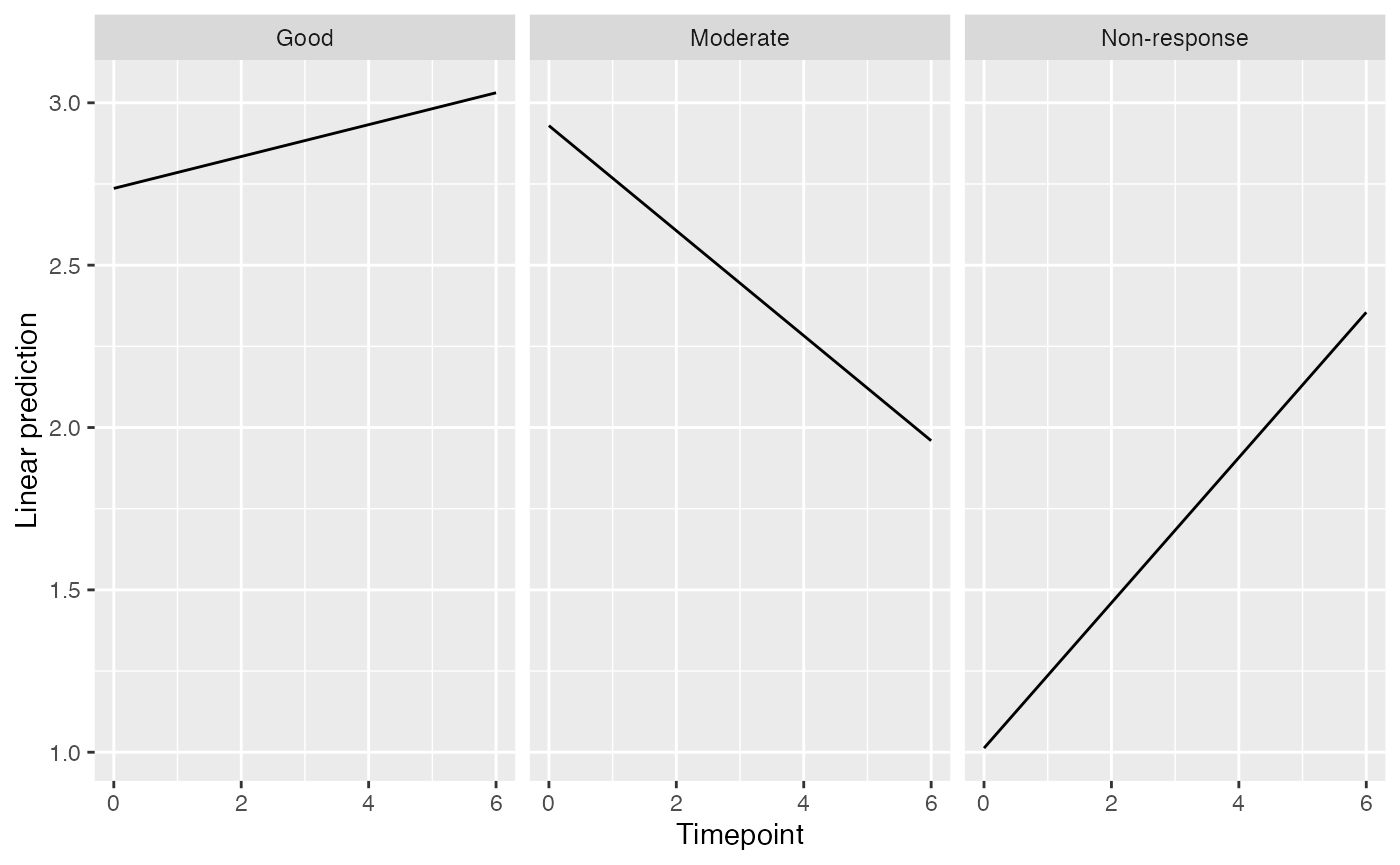

Refitting a different model

glmmRefit() allows a different model to be fitted using the original data. The example below shows how to refit the model without the interaction term and then perform a likelihood ratio test using anova. Note for glmmSeq() objects the LHS of the reduced formula must be "count", while for lmmSeq() objects the LHS must be "gene". For glmmTMB analyses, the GLM family can also be changed.

fit2 <- glmmRefit(results, gene = "MS4A1",
                  formula = count ~ Timepoint + EULAR_6m + (1 | PATID))

anova(fit, fit2)

## Data: data
## Models:
## fit2: count ~ Timepoint + EULAR_6m + (1 | PATID)
## fit: count ~ Timepoint + EULAR_6m + (1 | PATID) + Timepoint:EULAR_6m
##      npar    AIC    BIC  logLik deviance  Chisq Df Pr(>Chisq)  
## fit2    6 899.53 916.41 -443.77   887.53                       
## fit     8 898.68 921.18 -441.34   882.68 4.8505  2    0.08846 .
## ---
## Signif. codes:  0 '***' 0.001 '**' 0.01 '*' 0.05 '.' 0.1 ' ' 1

Model Plots

For variables such as time, which are matched according to an ID (the random effect), we can examine the fitted model using plots which show estimated means and confidence intervals based on coefficients for the fitted regression model, overlaid upon the underlying data. In this case the samples are matched longitudinally over time.

Plots can be viewed using either ggplot or base graphics. We can start looking at the gene with the most significant interaction IGHV3-23:

plotColours <- c("skyblue", "goldenrod1", "mediumseagreen")
modColours <- c("dodgerblue3", "goldenrod3", "seagreen4")
shapes <- c(17, 19, 18)

ggmodelPlot(results,
            geneName = "IGHV3-23",
            x1var = "Timepoint",
            x2var="EULAR_6m",
            xlab="Time",
            colours = plotColours,
            shapes = shapes,
            lineColours = plotColours, 
            modelColours = modColours,
            modelSize = 10)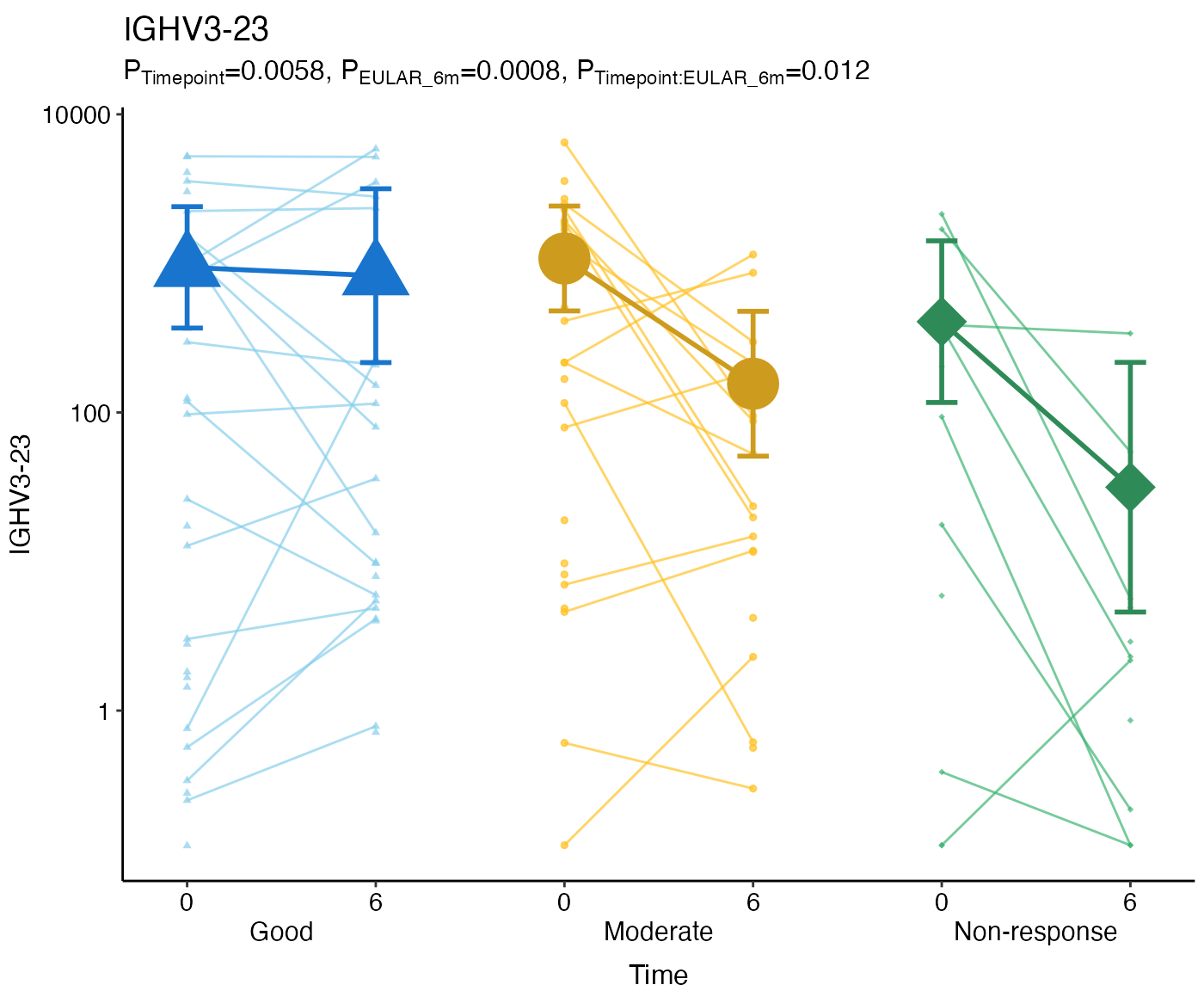

Alternatively plots can be generated using base graphics, here with or without the model fit overlaid. By default p-value labels are taken from the column names of the pvals object in the stats slot of the S4 result object. These can be relabelled using the plab argument.

oldpar <- par(mfrow=c(1, 2))

modelPlot(results2,
          geneName = "FGF14",
          x1var = "Timepoint",
          x2var="EULAR_binary",
          fontSize=0.65,
          colours=c("coral", "mediumseagreen"),
          modelColours = c("coral", "mediumseagreen"),
          modelLineColours = "black",
          modelSize = 2)

modelPlot(results,
          geneName = "EMILIN3",
          x1var = "Timepoint",
          x2var = "EULAR_6m",
          colours = plotColours,
          plab = c("time", "response", "time:response"),
          addModel = FALSE)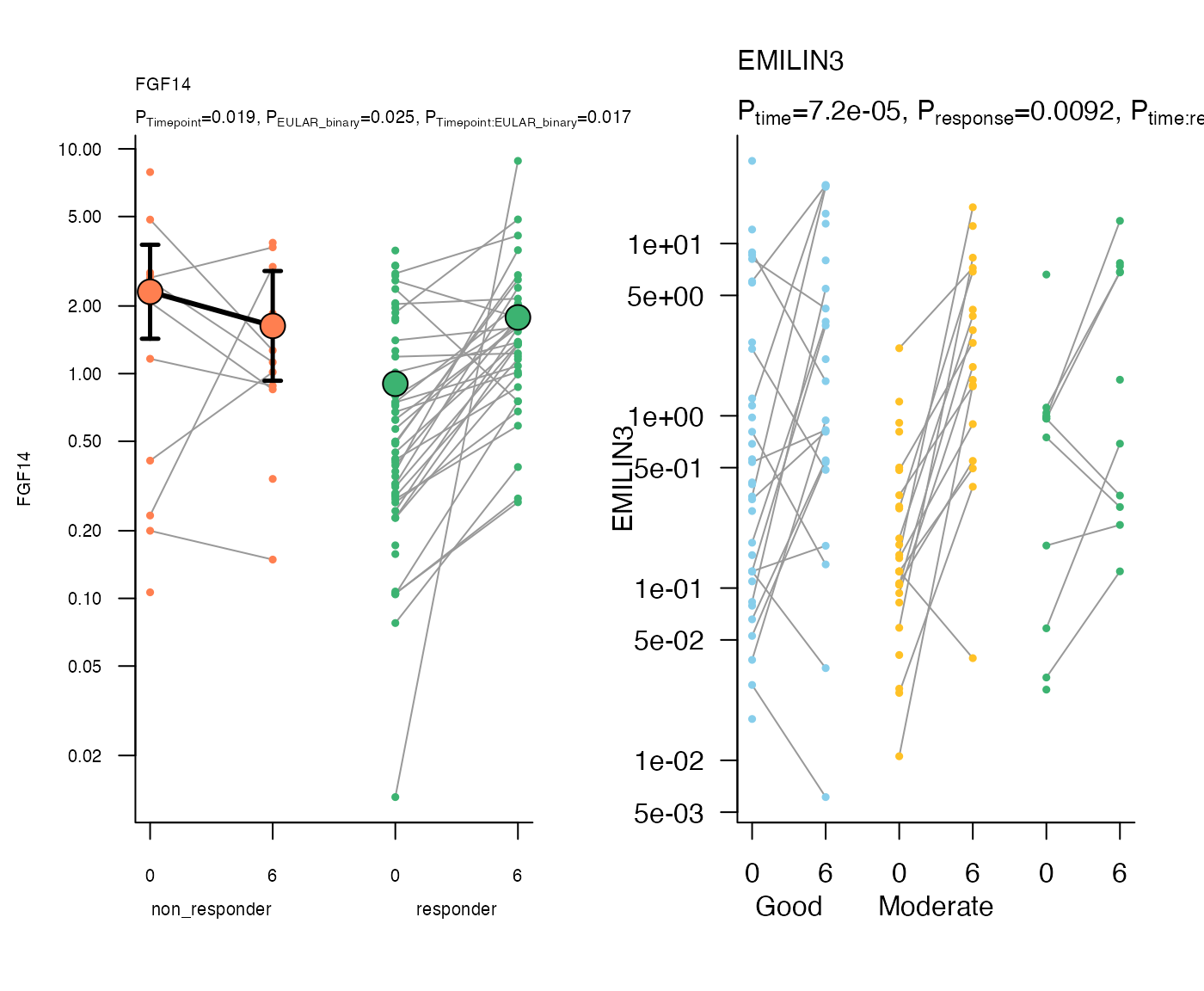

par(oldpar)

To plot the model fits alone set addPoints = FALSE.

library(ggpubr)

p1 <- ggmodelPlot(results,
                  "ADAM12",
                  x1var="Timepoint",
                  x2var="EULAR_6m",
                  xlab="Time",
                  addPoints = FALSE,
                  colours = plotColours)

p2 <- ggmodelPlot(results,
                  "EMILIN3",
                  x1var="Timepoint",
                  x2var="EULAR_6m",
                  xlab="Time",
                  fontSize=8,
                  x2Offset=1,
                  addPoints = FALSE,
                  colours = plotColours)

ggarrange(p1, p2, ncol=2, common.legend = T, legend="bottom")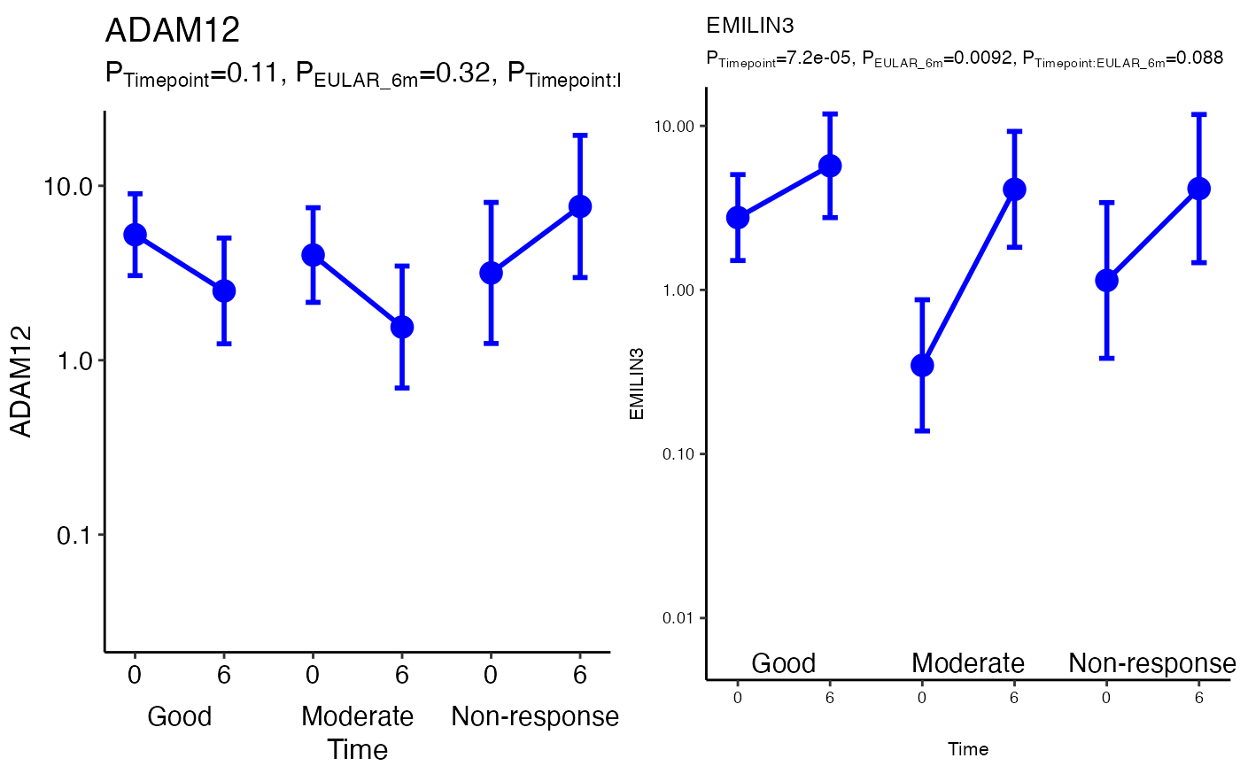

Fold change plots

The comparative fold change (for x1var variables) between conditions (x2var and x2Values variables) can be plotted using an fcPlot for all genes to highlight significance. This type of plot is most suited to look for interaction between time (x1var) and a two-level factor (x2var), looking at change between two timepoints. In the example below from the R4RA study [1], gene expression pre- and post-drug treatment is compared between two drugs (rituximab & tocilizumab), using the design formula gene_counts ~ time * drug. By setting graphics = "plotly" this can be viewed interactively.

r4ra_glmm <- glmmSeq(~ time * drug + (1 | Patient_ID), 
                       countdata = tpmdata, metadata,
                       dispersion = dispersions, cores = 8, removeSingles = T)
r4ra_glmm <- glmmQvals(r4ra_glmm)
labels = c(..)  # Genes to label
fcPlot(r4ra_glmm, x1var = "time", x2var = "drug", graphics = "plotly",
       pCutoff = 0.05, useAdjusted = TRUE,
       labels = labels,
       colours = c('grey', 'green3', 'gold3', 'blue'))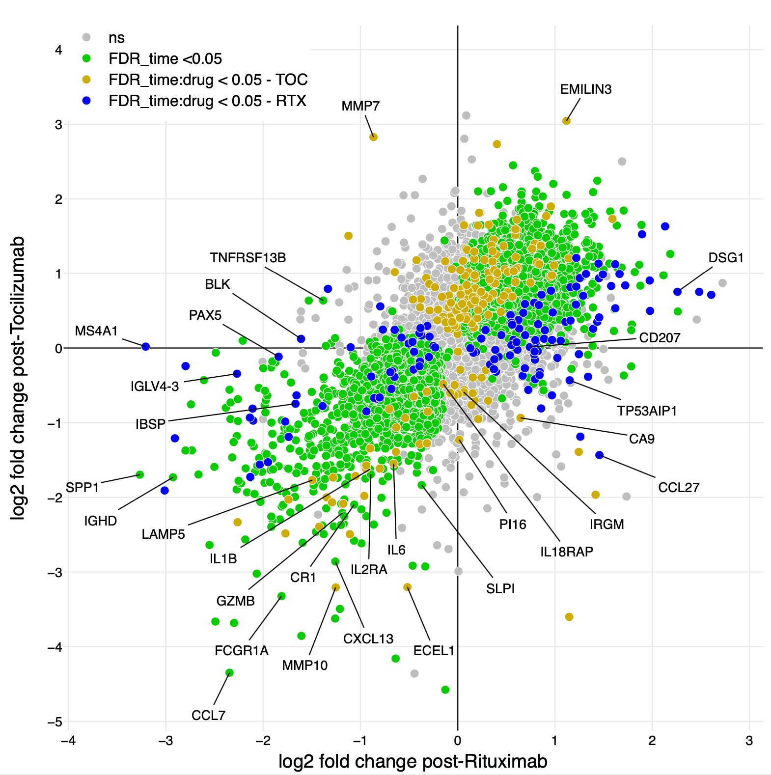

Log2 fold change between the two time points for individuals treated with rituximab on the x axis and individuals treated with tocilizumab on the y axis with each point representing a gene. Genes showing an interaction between time and drug are coloured blue or gold depending on whether their fold change is greater post-rituximab (blue) or post-tocilizumab (gold). Genes without interaction, but changing significantly over time are coloured green and tend to lie along the line of identity. See the Longitudinal tab in https://r4ra.hpc.qmul.ac.uk for an interactive version of the above plot.

MA plots

An MA plot is an application of a Bland–Altman plot. The plot visualizes the differences between measurements taken in two samples, by transforming the data onto M (log ratio) and A (mean average) scales, then plotting these values.

labels = c('MS4A1', 'FGF14', 'IL2RG', 'IGHV3-23', 'ADAM12', 'IL36G', 
           'BLK', 'SAA1', 'CILP', 'EMILIN3', 'EMILIN2', 'IGHJ6', 
           'CXCL9', 'CXCL13')
maPlots <- maPlot(results,
                  x1var="Timepoint",
                  x2var="EULAR_6m",
                  x2Values=c("Good", "Non-response"),
                  colours=c('grey', 'midnightblue',
                             'mediumseagreen', 'goldenrod'),
                  labels=labels,
                  graphics="ggplot")

maPlots$combined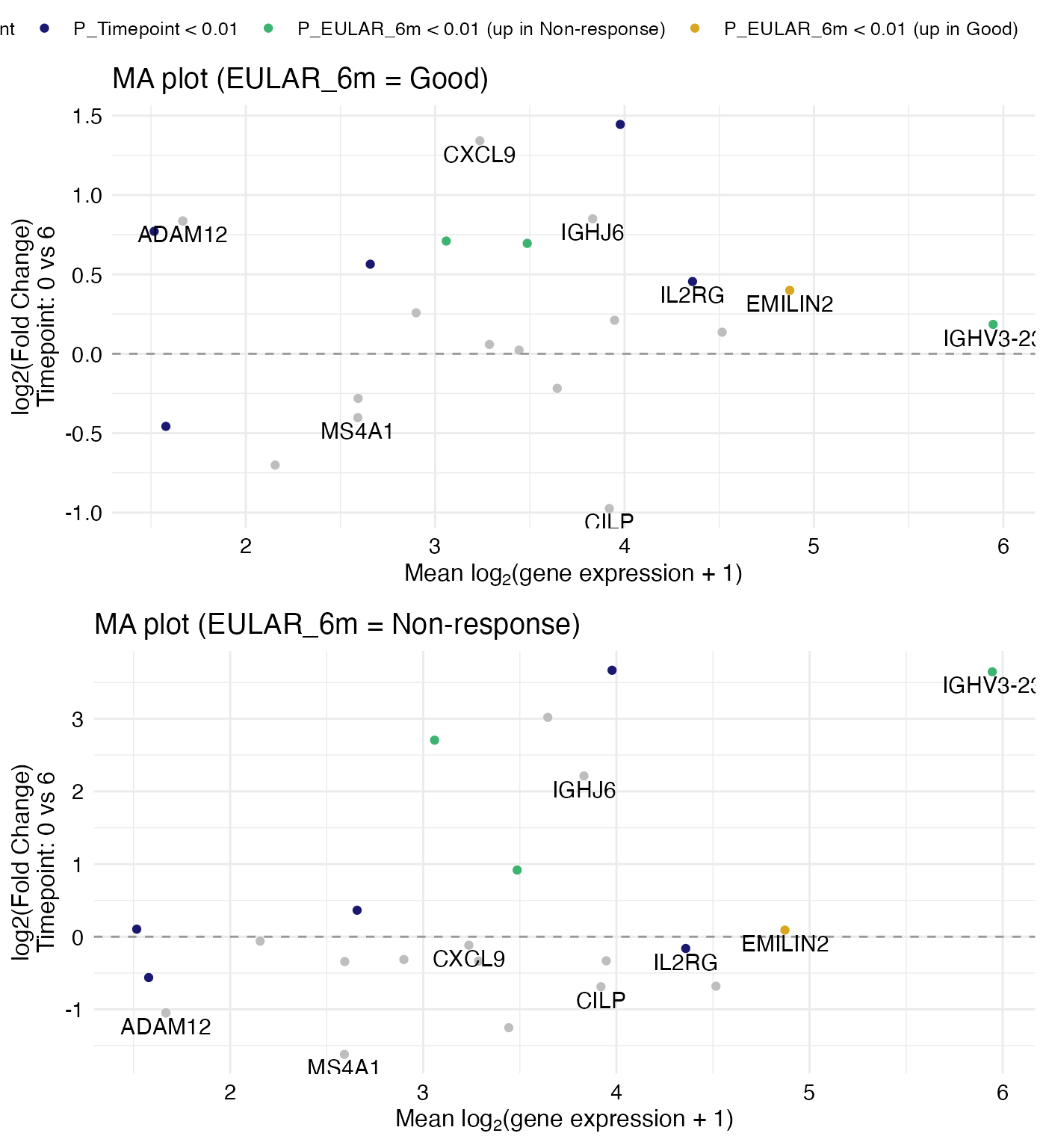

Troubleshooting

Mixed effects models are tricky to fit and lme4::glmer sometimes returns errors. In fact, a significant amount of code in glmmSeq is devoted to catching and handling errors to allow parallelisation to continue. Errors in genes are stored in the errors slot.

results@errors[1]   # first gene error

##                                                                                                                         IL12A 
## "Error in (function (fr, X, reTrms, family, nAGQ = 1L, verbose = 0L, maxit = 100L,  : \n  PIRLS loop resulted in NaN value\n"

Sometimes glmmSeq returns errors in all genes. This usually means a problem with not enough samples in each timepoint or a mistake in the formula. Since version 0.5.5 glmmSeq now returns a vector of the error messages for all genes, which can be useful for debugging. In the example below, only timepoint 0 is specified.

results3 <- glmmSeq(~ Timepoint * EULAR_6m + (1 | PATID),
                    countdata = tpm[, metadata$Timepoint == 0],
                    metadata = metadata[metadata$Timepoint == 0, ],
                    dispersion = disp)

## 
## n = 72 samples, 72 individuals

## All genes returned an error. Check call. Check sufficient data in each group

##                                                                              MS4A1 
## "fixed-effect model matrix is rank deficient so dropping 3 columns / coefficients"

If there are errors which are not caught by the error checking core mechanism, this can lead to problems with grouping results after the core models have been fit. Setting returnList=TRUE when calling glmmSeq returns the list output direct from mclapply (or parLapply on windows). This can be helpful for debugging unforeseeen problems in the core loop.

Citing glmmSeq

glmmSeq was developed by the bioinformatics team at the Experimental Medicine & Rheumatology department and Centre for Translational Bioinformatics at Queen Mary University London.

If you use this package please cite as:

citation("glmmSeq")

## 
## To cite package 'glmmSeq' in publications use:
## 
##   Lewis M, Goldmann K, Sciacca E (????). _glmmSeq: General Linear Mixed Models
##   for Gene-Level Differential Expression_. R package version 0.5.5,
##   <https://github.com/myles-lewis/glmmSeq>.
## 
## A BibTeX entry for LaTeX users is
## 
##   @Manual{,
##     title = {glmmSeq: General Linear Mixed Models for Gene-Level Differential Expression},
##     author = {Myles Lewis and Katriona Goldmann and Elisabetta Sciacca},
##     note = {R package version 0.5.5},
##     url = {https://github.com/myles-lewis/glmmSeq},
##   }

References

Felice Rivellese, Anna Surace, Katriona Goldmann, Elisabetta Sciacca, Cankut Cubuk, Giovanni Giorli, … Michael Barnes, Myles J. Lewis, Costantino Pitzalis, R4RA collaborative group. Rituximab versus tocilizumab in rheumatoid arthritis: synovial biopsy-based biomarker analysis of the phase 4 R4RA randomized trial. Nature medicine 2022; 28(6): 1256-68. doi:10.1038/s41591-022-01789-0

Statistical software used in this package:

lme4: Douglas Bates, Martin Maechler, Ben Bolker, Steve Walker (2015). Fitting Linear Mixed-Effects Models Using lme4. Journal of Statistical Software, 67(1), 1-48. doi: 10.18637/jss.v067.i01.
car: John Fox and Sanford Weisberg (2019). An {R} Companion to Applied Regression, Third Edition. Thousand Oaks CA: Sage. URL: https://socialsciences.mcmaster.ca/jfox/Books/Companion/
MASS: Venables, W. N. & Ripley, B. D. (2002) Modern Applied Statistics with S. Fourth Edition. Springer, New York. ISBN 0-387-95457-0
glmmTMB: Mollie Brooks, Ben Bolker, Kasper Kristensen, Martin Maechler, Arni Magnusson (2022). glmmTMB: Generalized Linear Mixed Models using Template Model Builder
qvalue: John D. Storey, Andrew J. Bass, Alan Dabney and David Robinson (2020). qvalue: Q-value estimation for false discovery rate control. R package version 2.22.0. https://github.com/StoreyLab/qvalue
lmerTest: Alexandra Kuznetsova, Per Brockhoff, Rune Christensen, Sofie Jensen. lmerTest: Tests in Linear Mixed Effects Models
emmeans: Russell V. Lenth, Paul Buerkner, Maxime Herve, Jonathon Love, Fernando Miguez, Hannes Riebl, Henrik Singmann. emmeans: Estimated Marginal Means, aka Least-Squares Means

glmmSeq

Myles Lewis, Katriona Goldmann, Elisabetta Sciacca, Cankut Cubuk, Anna Surace

2022-10-08

glmmSeq

Installing from CRAN

Installing from Github

Installing Locally

Overview

Metadata

Count data

Dispersion

Size Factors

Fitting Models

Outputs

Q-values

glmmTMB models

Gaussian mixed effects models

Hypothesis testing

Extracting individual Genes

Refitting a different model

Model Plots

Fold change plots

MA plots

Troubleshooting

Citing glmmSeq

References